Analyzing Categorical VAE Latent Space with NPMI

Intro

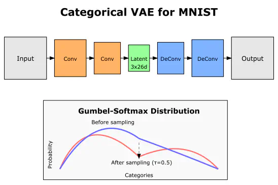
In my PhD thesis I made a claim that the NPMI method presented in our NeurIPS paper can be extended to other architectures, such as autoencoders, as they are, in essence, the same setup as the basic emergent communication agents. So to verify my own claim I wrote a very basic analysis of the latent space of a categorical VAE trained on MNIST. While there is almost certainly more to the latent space representation, even with some very basic code, I could potentially identify some patterns in how the data is represented.

Below is the annotated Jupyter Notebook code, which is also available in my GitHub repo here.

Wait, what is NPMI?

Normalized Pointwise Mutual Information (NPMI) is a normalized version of the Pointwise Mutual Information (PMI) collocation measure from linguistics. NPMI is particularly useful because it provides a more intuitive way to threshold significant correlations. Its values are conveniently bounded between -1 and 1:

• Negative values indicate negative correlation
• Zero indicates random association
• Values close to 1 indicate strong association between the latent representation and context

The diagram below illustrates these relationships:

Prep

Okay, so let’s start with the prep for actually analysing a latent space of a VAE.

First we need to import all the things that we will be using to both build the model, as well as analyse the latent space.

from collections import defaultdict, Counter
import torchvision.transforms as transforms
import torchvision
import torch
from models import Encoder, Decoder, CategoricalVAE
from models import gumbel_softmax
import itertools
from tqdm import tqdm
import numpy as np

To analyse the representation we will run through the whole MNIST dataset, and see what representation are used for each image.

transform = transforms.Compose([transforms.ToTensor()])
training_images = torchvision.datasets.MNIST(
    root="./data", train=True, transform=transform, download=True
)

We create the dataloader and load the model of the VAE (available in the repo here). For convenience, I use similar latent space parameters to the emergent communication NPMI paper.

batch_size = 1
train_dataset = torch.utils.data.DataLoader(
    dataset=training_images, batch_size=batch_size, shuffle=True
)

image_shape = next(iter(train_dataset))[0][0].shape  # [1, 28, 28]
K = 26  # number of classes
N = 3  # number of categorical distributions

encoder = Encoder(N, K, image_shape)
decoder = Decoder(N, K, image_shape)
model = CategoricalVAE(encoder, decoder)

state_dict = torch.load("outputs/default/save_49999.pt", weights_only=True)
model.load_state_dict(state_dict)

Gathering the data

Now we can get to building the dataset for our analysis!

We run every single image through our VAE, and extract:

1. The Gumbel-Softmax latent space representation
2. The label of the image

To make this analysis more general, instead of the label we would use things like presence of lines, diagonals etc. This way the method does not need to rely on any dataset labelling, but instead on features present and/or extracted from the dataset. But for this simple example we just use the dataset labels.

latents = []
labels = []
for batch in tqdm(train_dataset):
    with torch.no_grad():
        phi, x_hat = model(batch[0], temperature=1.0)
        z_given_x = gumbel_softmax(phi, temperature=1.0, hard=True, batch=True)
        latents.append(z_given_x.argmax(axis=2)[0].numpy())
        labels.append(batch[1].item())

Building the probabilities

For the NPMI analysis we will need to know three things:

• Probability of a given latent space representation being used
• Probability of a given observation occurring
• Joint probability of the above

Then we can calculate the NPMI using the formula:

This formula combines the PMI with the joint self-information $h$, providing a normalized measure of association.

total = len(labels)
obs_probs = {k:v/total for k,v in dict(Counter(labels)).items()}

latents_uniq, counts =  np.unique(latents,axis=0,return_counts=True)

joint_probs = defaultdict(lambda: defaultdict(int))
for latent_id in tqdm(range(latents_uniq.shape[0])):
    for idx, latent in enumerate(latents):
        if np.array_equal(latent,latents_uniq[latent_id]):
            joint_probs[latent_id][labels[idx]] += 1

for latent_id in tqdm(range(latents_uniq.shape[0])):
    for obs_type in joint_probs[latent_id].keys():
        joint_probs[latent_id][obs_type] /= total

Calculating NPMI and getting the colocations

np.seterr(divide="ignore", invalid="ignore")

for latent_id in range(latents_uniq.shape[0]):
    latent_prob = counts[latent_id]/total
    for obs_type in list(obs_probs.keys()):
        obs_prob = obs_probs[obs_type]
        joint_prob = joint_probs[latent_id][obs_type]
        joint_self_information = -np.log2(joint_prob)
        npmi = np.log2(joint_prob / (latent_prob * obs_prob)) / joint_self_information
        if npmi > 0.3:
            print(f"Possible hit for latent {latents_uniq[latent_id]} and observation type {obs_type}")

Possible hit for latent [0 1 7] and observation type 1
Possible hit for latent [ 0 12 25] and observation type 5
Possible hit for latent [ 0 14  5] and observation type 2
Possible hit for latent [ 0 18 23] and observation type 1
Possible hit for latent [ 0 19  8] and observation type 4
.....

With a threshold of $0.3$, we got a LOT of possible hits. So to narrow it down to most likely candidates we can increase the threshold to $0.4$

for latent_id in range(latents_uniq.shape[0]):
    latent_prob = counts[latent_id]/total
    for obs_type in list(obs_probs.keys()):
        obs_prob = obs_probs[obs_type]
        joint_prob = joint_probs[latent_id][obs_type]
        joint_self_information = -np.log2(joint_prob)
        npmi = np.log2(joint_prob / (latent_prob * obs_prob)) / joint_self_information
        if npmi > 0.4:
            print(f"Possible hit for latent {latents_uniq[latent_id]} and observation type {obs_type}")

Possible hit for latent [ 3 13 18] and observation type 1
Possible hit for latent [ 3 13 23] and observation type 1
Possible hit for latent [25 13  7] and observation type 1
Possible hit for latent [25 13 23] and observation type 1
Possible hit for latent [25 18 23] and observation type 1
.....

Now we can even see some patterns. While the simple method presented in this post uses only monolithic latent representation, perhaps if we scaled this up, we could find some compositional structure to the latent space. For example, $13$ in the second position of the representation could mean a diagonal line, so could also be present in images of the number 7.

I hope this illsutrate just how powerful NPMI can be for analysing latent spaces of any model. As long as we can observe the inputs and the latent representations, we can potentially build an understanding of how models store information. This could also be applied to intermediate layers to understand how such information is being built upon!